01The gap between two witnesses
Every storage workload has two witnesses to the same events, and neither tells the whole truth alone. The application knows intent — "these 2.6 MB of node features are what I actually consume." The device knows mechanism — "1140 MB of 4 KiB pages crossed the PCIe bus." Read amplification is the gap between them.
A GNN that offloads node features to an SSD is the textbook case. Each feature vector is 17 floats — 68 bytes. But storage is paged: a single scattered neighbor drags a whole 4 KiB page for that 68 bytes. Sample a batch of neighbors that land on 240,000 different pages and the device moves a gigabyte to feed a workload that consumes a couple of megabytes. The in-RAM counter can model this; eBPF at the nvme tracepoints proves it — and here the device-side count matched the store's own read count to the command (240,698 vs 240,698 reads).
◱intent witness
The driver emits its useful
feature bytes on a CLOCK_MONOTONIC axis — what the GNN actually consumes.
▣mechanism witness
nvme_tp_monitor
records every device command on the same clock — slba, bytes, completion latency. No
user_data needed; this is plain O_DIRECT block IO.
⚲the gap is the story
Lay the two on one timeline and the read amplification is not a statistic — it is the visible distance between two curves.
02The A/B: naive access vs the architectural fix
The same features, the same SSD, the same 3.7M-node graph. The only thing that changes is the access pattern. NeighborLoader samples neighbors and reads each one's page individually. Page-Aware batching — a knlp engineering fix — reads pages whole and uses every node on them. That one change cuts device traffic ~50× for the identical GNN signal, and it generalizes to any GNN (or KV cache) that offloads to storage.
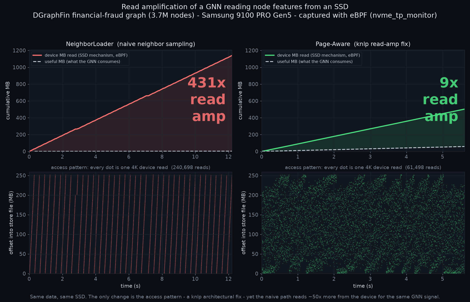
| arm | useful (intent) | device read (eBPF) | RA_signal | RA_fetch |
|---|---|---|---|---|
| NeighborLoader — naive neighbor sampling | 2.65 MB | 1140 MB · 240,698 reads | 431× | ~57× |
| Page-Aware — knlp read-amp fix | 58.3 MB | 502 MB · 61,498 reads | 8.6× | ~2× |
RA_signal = device bytes / useful feature bytes (vs what the model
consumes). RA_fetch = device bytes / minimal pages needed (the store's own
ra_physical: the page-granularity tax even after you account for necessary paging).
Both are honest; RA_signal is the end-to-end number a workload actually pays.
03What the Perfetto timeline shows
Drag gnn_readamp_dgraphfin_ab.pftrace.gz onto
ui.perfetto.dev (local WASM; nothing uploads). Each arm is a
process group rebased to t=0, so naive and page-aware sit side by side. Per arm:
| counter | what it shows |
|---|---|
| useful MB (intent) | the feature bytes the GNN consumes — the denominator of read amplification |
| device MB, store count | the store's own read accounting (intent side) |
| device MB, eBPF | the independent device-side truth — it tracks the store count, which is the capture verifying itself |
| read amplification × | device MB / useful MB, running: 431× vs 8.6× |
| device LBA (sector) | slba over time — the access pattern: scatter for poor locality, banded for good |
The useful curve sitting far below device is the amplification. The two device curves coinciding is the honesty check: the eBPF witness and the application's self-report agree, so the huge number is not an artifact of either one.
04Capture a confidential workload, share only the shape
This is why the capture matters beyond a pretty chart. A device capture — and the fio iolog made from it — carries only IO shape: operation, offset, length, timing. No feature values, no node ids, no graph, no keys.
So a third party can run their confidential GNN — real financial-fraud data,
private customer graph — capture it with these tracers, and hand back a trace or an iolog that we
replay and visualize to reproduce the exact device read pattern without ever seeing their
data. mk_dev_iolog.py turns the capture into a fio v3 iolog:
fio version 3 iolog
0 /dev/nvme0n1 add
0 /dev/nvme0n1 open
0 /dev/nvme0n1 read 3451445895168 4096
0 /dev/nvme0n1 read 3451445907456 4096
0 /dev/nvme0n1 read 3451445919744 4096
... 240,695 more reads: offset + length + time only ...Replayed read-only with fio --read_iolog --direct=1 and refereed against the
original capture by compare_streams.py, the reproduction is exact:
| commands | bytes | size mix | |
|---|---|---|---|
| original capture | 240,698 | 1140 MB | 4K:208136 8K:28196 12K:3749 |
| replay from iolog | 240,702 | 1140 MB | 4K:208138 8K:28198 12K:3749 |
| inflation | +0.0% | +0.0% | identical |
100% of the original commands reproduced at identical offset and size, from an artifact that contains none of the data.
05Reproduce it
Full recipe in tools/reproduce/gnn-readamp/. The shape of it:
# 1. capture both arms at the device layer (knlp force-SSD store, O_DIRECT)
./cap_ssd.sh neighbor natural 12 /tmp/nbr
./cap_ssd.sh page natural 12 /tmp/page
# 2. A/B onto one Perfetto timeline
python3 examples/replay/readamp2perfetto.py \
--arm "NeighborLoader (naive):/tmp/nbr.jsonl:/tmp/nbr.phase.txt" \
--arm "Page-Aware (knlp fix):/tmp/page.jsonl:/tmp/page.phase.txt" \
-o gnn_readamp_ab.pftrace
# 3. data-free replay + fidelity referee
python3 examples/replay/mk_dev_iolog.py /tmp/nbr_reads.jsonl /dev/nvme0n1 > nbr.iolog
sudo fio --name=replay --filename=/dev/nvme0n1 --readonly --direct=1 \
--ioengine=psync --read_iolog=nbr.iolog06Where the pieces live
Two trees, one boundary. The tools and this value showcase live in ebpf-syscall; the ready-to-view demo trace lives in the gallery as a data artifact.
- ebpf-syscall — the tracer (
nvme_tp_monitor), the converter (examples/replay/readamp2perfetto.py), the replay tools (mk_dev_iolog.py,compare_streams.py), the reproduce recipe (tools/reproduce/gnn-readamp/), and this page. - kvio-perfetto-gallery — the draggable
traces/gnn_readamp_dgraphfin_ab.pftrace.gzplus its figure and machine-readable report. A demo artifact; it links back here for the story.